
“DO NOT GO GENTLE IN THE DARK”
不知不觉又踏入了人工智能的领域
在这里提醒自己不要忘了学习的初衷: 一切为安全
希望能够将学习到的人工智能方面的知识,包括深度学习、神经网络等应用到网络安全领域
回归问题实例
思路梳理:
初始化学习参数:
learning_rate = 0.0001 #学习率
initial_b = 0 #初始b值
initial_w = 0 #初始w值
num_iterations = 10000 #迭代次数
points [x, y] #使用的点数据
计算初始数据的损失
- compute_error_for_line_given_points(initial_b, initial_w …)
梯度下降计算
- gradient_descent_runner(points, initial_b, initial_w, learning_rate, num_iterations)
- step_gradient(b, w, np.array(points), learning_rate)
- gradient_descent_runner(points, initial_b, initial_w, learning_rate, num_iterations)
1 | import numpy as np |
代码备注:
“data.csv”使用np生成的一个x,y坐标数据,生成代码如下:
- np.random.rand() 生成的数据服从均值为0,方差为1的正态分布
1
2
3
4
5
6
with open("data.csv", "w", newline="") as file:
writer = csv.writer(file)
for i in range(100):
x = np.random.rand() * 100
y = np.random.rand() * 100
writer.writerow([x, y])
Tensor
torch.FloatTensor
用于生成数据类型为浮点的tensor,入参可以是列表,也可以是一个维度值
torch.range(起始值,结束值,步长)
搭建一个简易的神经网络
- 简介:
1 | 1.设置输入节点为1000,隐藏层的节点为100,输出层的节点为10 |
- 代码:
1 | batch_n = 100 #一个批次输入的数据量 |
搭建一个较完整的神经网络
代码:
1
2
3
4
5
6
7
8
9
10
11
12
13
14
15
16
17
18
19
20
21
22
23
24
25
26
27
28
29
30
31
32
33
34
35
36
37
38
39
40
41batch_n = 100 # 输入的数据量
input_data = 1000 # 每个数据的特征数量
hidden_layer = 100 # 隐藏层的神经元数量
output_data = 10 # 输出为的特征量的个数
'''
自动梯度的功能过程大致为:先通过输入的Tensor数据类型的变量在神经网络的前向传播过程中生成一张计算图,
然后根据这个计算图和输出结果精确计算出每一个参数需要更新的梯度,并通过完成后向传播完成对参数的梯度更新。
完成自动梯度需要用到的torch.autograd包中的Variable类对我们定义的Tensor数据类型变量进行封装,
在封装后,计算图中的各个节点就是一个Variable对象,这样才能应用自动梯度的功能。
'''
'''
#用Variable对Tensor数据类型变量进行封装的操作。
requires_grad如果是False,表示该变量在进行自动梯度计算的过程中不会保留梯度值。
'''
x = Variable(torch.randn(batch_n, input_data), requires_grad=False)
y = Variable(torch.randn(batch_n, output_data), requires_grad=False)
w1 = Variable(torch.randn(input_data, hidden_layer), requires_grad=True)
w2 = Variable(torch.randn(hidden_layer, output_data), requires_grad=True)
epoch_n = 50 # 迭代次数
lr = 1e-6 # 学习率
for epoch in range(epoch_n):
h1 = x.mm(w1) # 隐藏网络的净活性
print(h1.shape)
h1 = h1.clamp(min=0)
y_pred = h1.mm(w2) # 预计的输出值 也是隐藏网络的活性值
loss = (y_pred - y).pow(2).sum() # 损失函数
print("epoch:{},loss:{:.4f}".format(epoch, loss))
loss.backward() # 后向传播
w1.data -= lr * w1.grad.data
w2.data -= lr * w2.grad.data
w1.grad.data.zero_()
w2.grad.data.zero_()
torch.nn.Sequential类
- 备注:
1 | ''' |
代码:
1
2
3
4
5
6
7
8
9
10
11
12batch_n = 100 # 输入的数据量
input_data = 1000 # 每个数据的特征数量
hidden_layer = 100 # 隐藏层的神经元数量
output_data = 10 # 输出为的特征量的个数
x = Variable(torch.randn(batch_n, input_data), requires_grad=False)
y = Variable(torch.randn(batch_n, output_data), requires_grad=False)
models = torch.nn.Sequential(
torch.nn.Linear(input_data, hidden_layer),
torch.nn.ReLU(),
torch.nn.Linear(hidden_layer, output_data)
)
torch.nn.MSELoss类
介绍:
使用均方误差函数对损失值进行计算,定义类的对象时不用传入任何参数,但在使用实例时需要输入两个维度一样的参数方可进行计算
代码:
1
2
3
4
5loss_f = torch.nn.MSELoss()
x = Variable(torch.randn(100, 100))
y = Variable(torch.randn(100, 100))
loss = loss_f(x, y)
print(loss.data)
使用损失函数的神经网络
代码
1
2
3
4
5
6
7
8
9
10
11
12
13
14
15
16
17
18
19
20
21
22
23
24
25
26
27
28loss_f = torch.nn.MSELoss()
batch_n = 100
input_data = 1000
hidden_layer = 100
output_data = 10
epoch_n = 10000
lr = 1e-6
x = Variable(torch.randn(batch_n, input_data), requires_grad=False)
y = Variable(torch.randn(batch_n, output_data), requires_grad=False)
models = torch.nn.Sequential(
torch.nn.Linear(input_data, hidden_layer),
torch.nn.ReLU(),
torch.nn.Linear(hidden_layer, output_data)
)
for epoch in range (epoch_n):
y_pred = models(x)
loss = loss_f(y_pred, y)
if epoch % 1000 == 0:
print("epoch:{},loss:{:.4f},".format(epoch, loss.data))
models.zero_grad()
loss.backward()
for param in models.parameters():
param.data -= param.grad.data * lr
torch.optim包
提供非常多的可实现参数自动优化的类,如SGD、AdaGrad、RMSProp、Adam等
使用自动优化的类实现神经网络:
1 | batch_n = 100 # 一个批次输入数据的数量 |
实例:预测房价
根据历史数据预测未来的房价,实现一个线性回归模型,并用梯度下降算法求解该模型,从而给出预测直线、
求解步骤:准备数据、设计模型、训练和预测
1.准备数据
1 |
|
2.设计模型
- 希望的到一条尽可能从中间穿越这些数据散点的拟合直线
- 损失函数
- 梯度下降
- 学习率
3.训练
1 | # 定义随机的a b (线性方程的两个参数,斜率和偏置) |
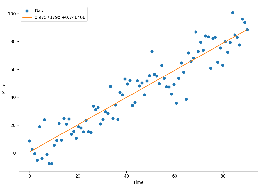
4.画出拟合直线
1 | x_data = x_train.data.numpy() # 将x中的数据转换成numpy数组 |
效果如下:
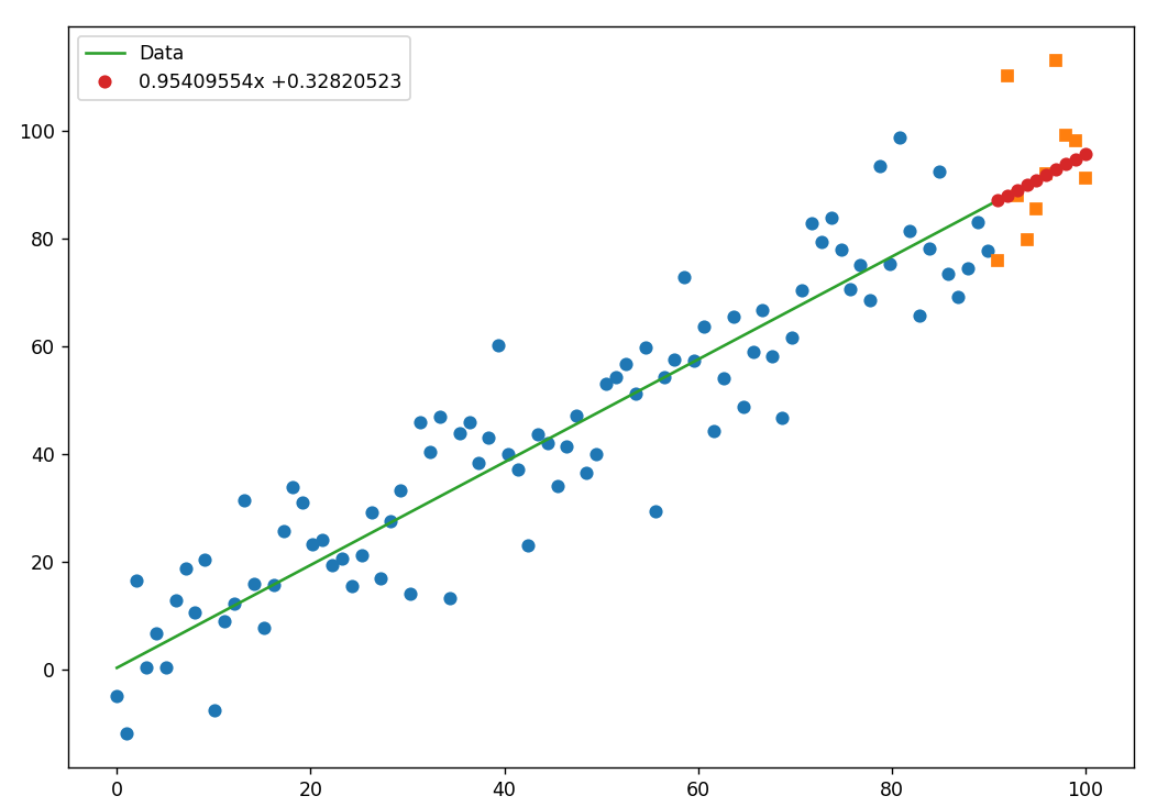
5.模型预测
1 | predictions = a.expand_as(x_test) * x_test + b.expand_as(x_test) |
效果如下:
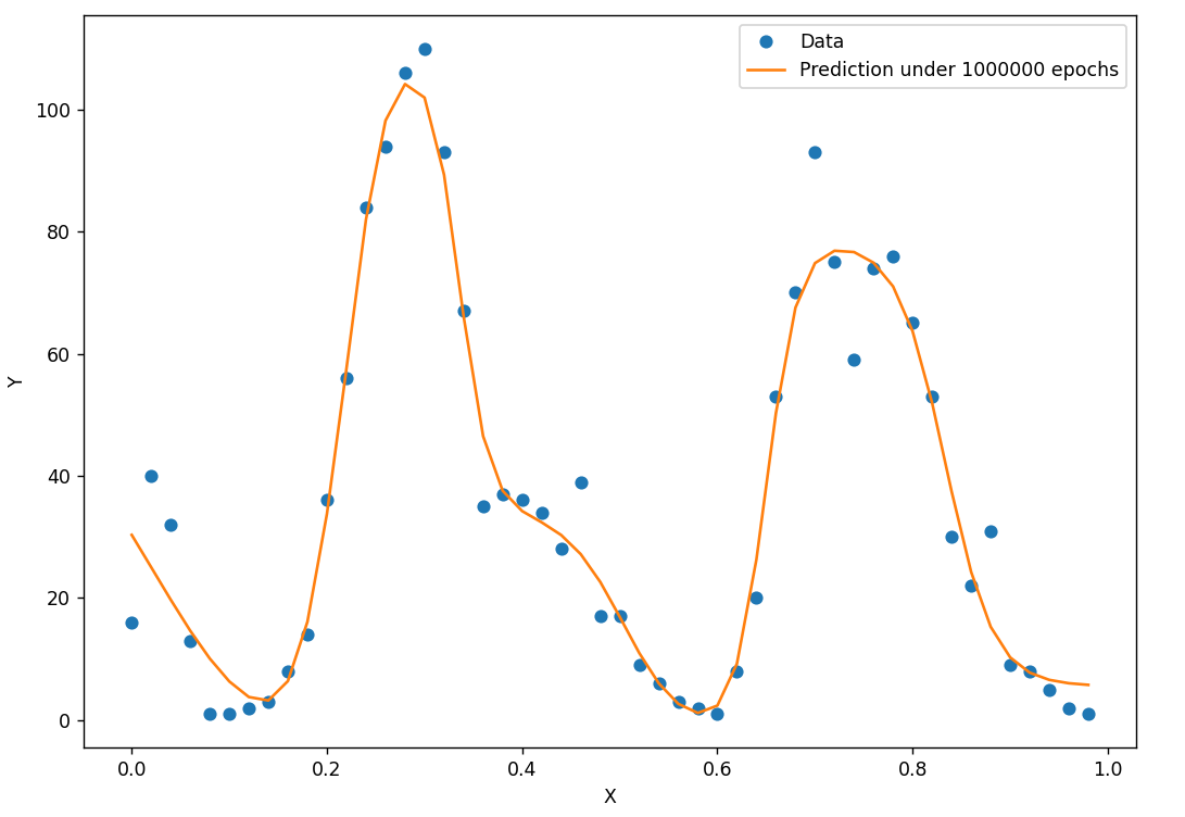
单车预测器
1.0:使用时间变量x作为自变量
1 | import inline |
训练效果
数据拟合曲线:
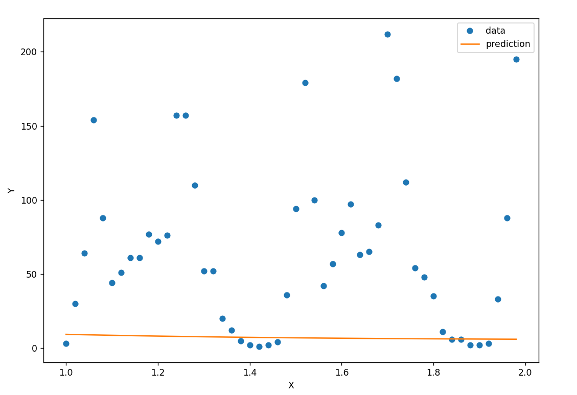
预测效果: 由于使用的自变量x和Y之间不存在依赖关系,得到的模型完全失能
预测曲线如下:
2.0 使用相关数据预测
1 | ''' |
中文情绪分类器
1 |
|
卷积神经网络
实现手写数字识别
1 | # _*_ coding : utf-8_*_ |
注:由于博客篇幅过长,后续的模块可能会单独写一个博客总结。详见分类——机器学习